Entities

This section introduces the different entities that can be created and stored in the geoh5 file format.

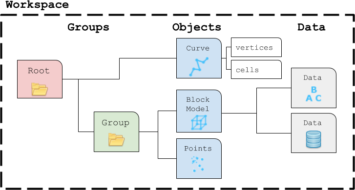
Groups

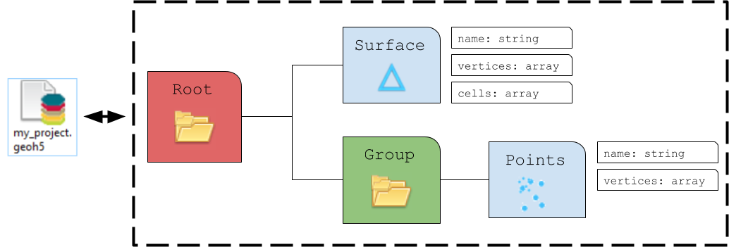
Groups are effectively containers for other entities, such as Objects (Points, Curve, Surface, etc.) and other Groups. Groups are used to establish parent-child relationships and to store information about a collection of entities.

RootGroup

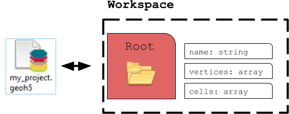
By default, the parent of any new Entity is the workspace RootGroup. It is the only entity in the Workspace without a parent. Users rarely have to interect with the Root group as it is mainly used to maintain the overall project hierarchy.

ContainerGroup

A ContainerGroup can easily be added to the workspace and can be assigned a name and description.

from geoh5py.groups import ContainerGroup
from geoh5py.workspace import Workspace
import numpy as np

# Create a blank project
workspace = Workspace("my_project.geoh5")

# Add a group
group = ContainerGroup.create(workspace, name='myGroup')

At creation, "myGroup" is written to the project geoh5 file and visible in the Analyst project tree.

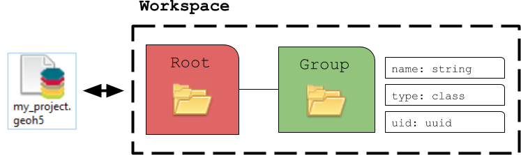
Any entity can be accessed by its name or uid (unique identifier):

print(group.uid)
print(workspace.get_entity("myGroup")[0] == workspace.get_entity(group.uid)[0])

15693108-e55e-4321-acde-957f1bccfa9e
True

Objects

The geoh5 format enables storing a wide variety of Object entities that can be displayed in 3D. This section describes the collection of Objects entities currently supported by geoh5py.

Points

The Points object consists of a list of vertices that define the location of actual data in 3D space. As for all other Objects, it can be created from an array of 3D coordinates and added to any group as follow:

from geoh5py.objects import Points

# Generate a numpy array of xyz locations
n = 100
radius, theta = np.arange(n), np.linspace(0, np.pi*8, n)

x, y = radius * np.cos(theta), radius * np.sin(theta)
z = (x**2. + y**2.)**0.5
xyz = np.c_[x.ravel(), y.ravel(), z.ravel()] # Form a 2D array

# Create the Point object
points = Points.create(
    workspace,       # The target Workspace
    vertices=xyz     # Set vertices
)

Curve

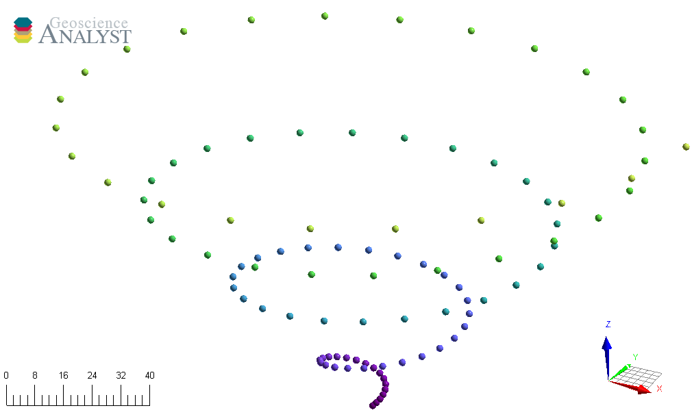
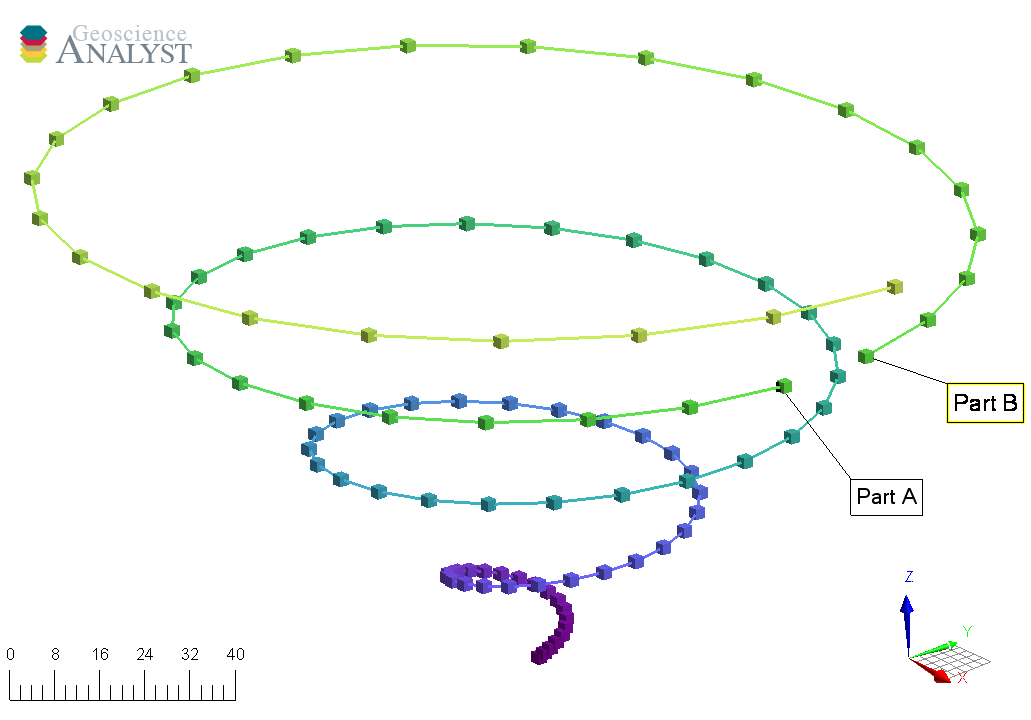
The Curve object, also known as a polyline, is often used to define contours, survey lines or geological contacts. It is a sub-class of the Points object with the added cells property, that defines the line segments connecting its vertices. By default, all vertices are connected sequentially following the order of the input vertices.

from geoh5py.objects import Curve

# Create the Curve object
curve = Curve.create(
    workspace,       # The target Workspace
    vertices=xyz
)

Alternatively, the cells property can be modified, either directly or by assigning parts identification to each vertices:

# Split the curve into two parts
part_id = np.ones(n, dtype="int32")
part_id[:75] = 2

# Assign the part
curve.parts = part_id

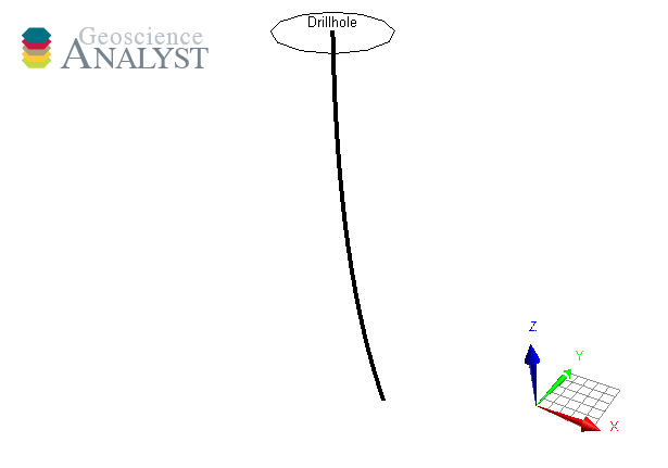
Drillhole

Drillhole objects are different from other objects as their 3D geometry is defined by the collar and surveys attributes. As for version geoh5 v2.0, the drillholes require a DrillholeGroup entity to store the geometry and data.

from geoh5py.groups import DrillholeGroup
from geoh5py.objects import Drillhole

dh_group = DrillholeGroup.create(workspace)

# Create a simple well
total_depth = 100
dist = np.linspace(0, total_depth, 10)
azm = np.ones_like(dist) * 45.
dip = np.linspace(-89, -75, dist.shape[0])
collar = np.r_[0., 10., 10]

well = Drillhole.create(
    workspace, collar=collar, surveys=np.c_[dist, azm, dip], name="Drillhole", parent=dh_group
)

print(well.name)

Drillhole

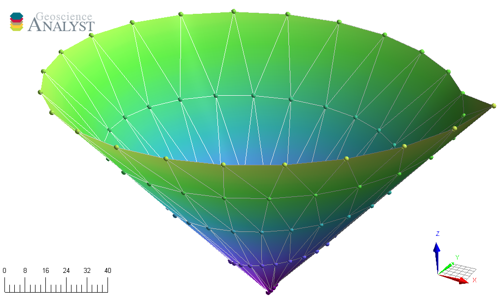
Surface

The Surface object is also described by vertices and cells that form a net of triangles. If omitted on creation, the cells property is calculated using a 2D scipy.spatial.Delaunay triangulation.

from geoh5py.objects import Surface
from scipy.spatial import Delaunay

# Create a triangulated surface from points
surf_2D = Delaunay(xyz[:, :2])

# Create the Surface object
surface = Surface.create(
    workspace,
    vertices=points.vertices, # Add vertices
    cells=surf_2D.simplices
)

GeoImage

The GeoImage object handles raster data, either single or 3-band images.

from geoh5py.objects import GeoImage

geoimage = GeoImage.create(workspace)

Image values can be assigned to the object from either a 2D numpy.ndarray for single band (gray):

geoimage.image = np.random.randn(128, 128)
display(geoimage.image)

or as 3D numpy.ndarray for 3-band RGB image:

geoimage.image = np.random.randn(128, 128, 3)
display(geoimage.image)

or directly from file (png, jpeg, tiff).

geoimage.image = "./images/flin_flin_geology.jpg"

A PIL.Image object gets exposed to the user, which can be used for common raster manipulation (rotation, filtering, etc). The modified raster is stored back on file as a blob (bytes).

display(geoimage.image)

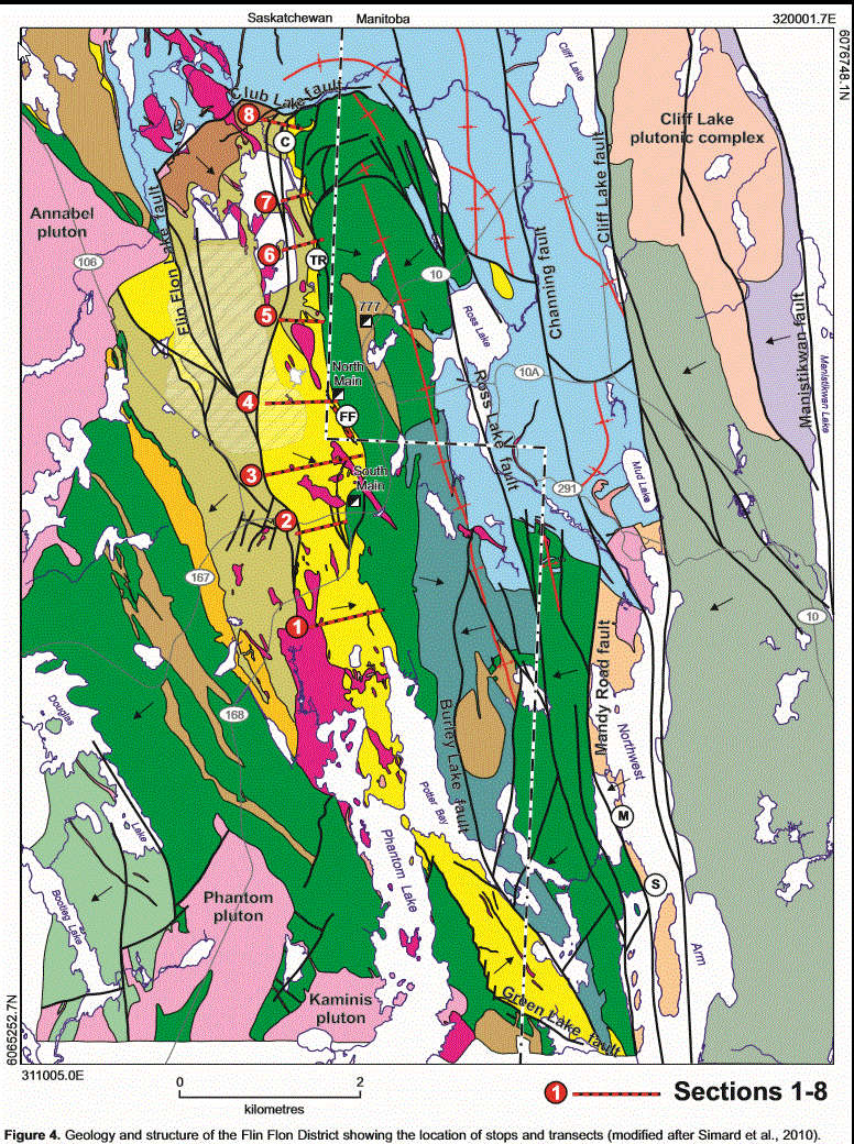
Geo-referencing

By default, the GeoImage object will be displayed at the origin (xy-plane) with dimensions equal to the pixel count. The utility function GeoImage.georeference lets users geo-reference the image in 3D space based on at least three (3) input reference points (pixels) with associated world coordinates.

pixels = [
    [18, 73],
    [757, 1014],
    [18, 1014],

]
coords = [
    [311005, 6065252, 0],
    [320001, 6076748, 0],
    [311005, 6076748, 0]
]

geoimage.georeference(pixels, coords)
print(geoimage.vertices)

[[ 310785.88227334 6077065.63655685       0.        ]
 [ 320232.29093369 6077065.63655686       0.        ]
 [ 320232.29093369 6064360.17428268       0.        ]
 [ 310785.88227334 6064360.17428268       0.        ]]

Grid2D

The Grid2D object defines a regular grid of cells often used to display model sections or to compute data derivatives. A Grid2D can be oriented in 3D space using the origin, rotation and dip parameters.

from geoh5py.objects import Grid2D

# Create the Surface object
grid = Grid2D.create(
    workspace,
    origin = [25, -75, 50],
    u_cell_size = 2.5,
    v_cell_size = 2.5,
    u_count = 64,
    v_count = 16,
    rotation = 90.0,
    dip = 45.0,
)

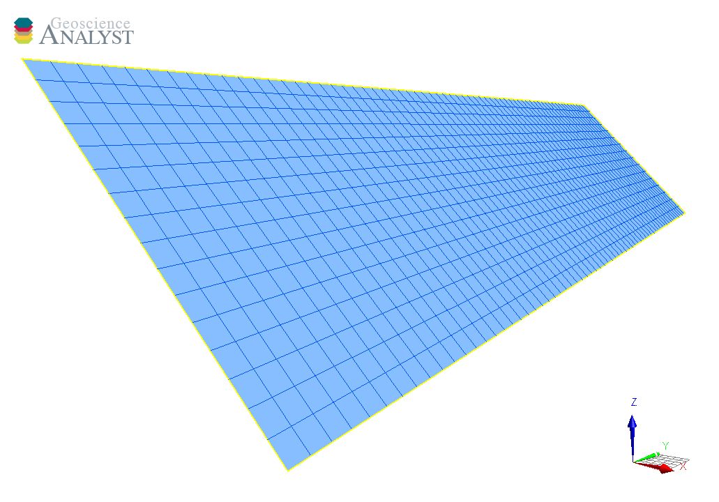
DrapeModel

The DrapeModel object defines an array of vertical (curtain) cells draped below a curved trace.

• The prisms attribute defines the elevation and position of the uppermost cell faces.

• The layers attribute defines the bottom face elevation of cells.

In the example below we create a simple DrapeModel object along a sinusoidal path with equal number of layers below every station. Variable number of layers per prism is also supported.

from geoh5py.objects import DrapeModel

# Define a simple trace
n_columns = 32
n_layers = 8

x = np.linspace(0, np.pi, n_columns)
y = np.cos(x)
z = np.linspace(0, 1, n_columns)

# Count the index and number of values per columns
layer_count = np.ones(n_columns) * n_layers
prisms = np.c_[
    x,
    y,
    z,
    np.cumsum(layer_count) - n_layers,
    layer_count
]

# Define the index and elevation of draped cells
k_index, i_index = np.meshgrid(np.arange(n_layers), np.arange(n_columns))
z_elevation = z[i_index] - np.linspace(0.5, 2, n_layers)

layers = np.c_[
    i_index.flatten(), k_index.flatten(), z_elevation.flatten()
]

# Create the object
drape = DrapeModel.create(workspace, prisms=prisms, layers=layers)

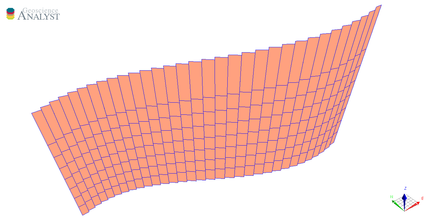
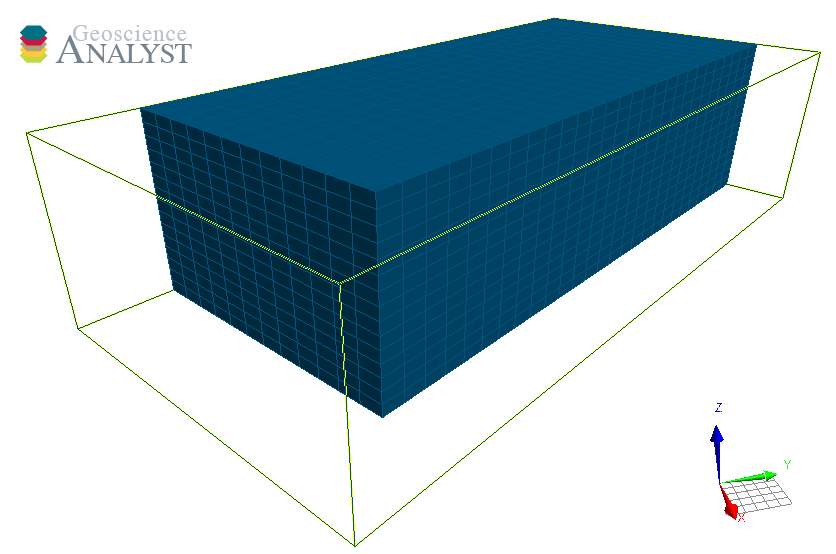
BlockModel

The BlockModel object defines a rectilinear grid of cells, also known as a tensor mesh. The cells center position is determined by cell_delimiters (offsets) along perpendicular axes (u, v, z) and relative to the origin. BlockModel can be oriented horizontally by controlling the rotation parameter.

from geoh5py.objects import BlockModel

# Create the Surface object
blockmodel = BlockModel.create(
    workspace,
    origin = [25, -100, 50],
    u_cell_delimiters=np.cumsum(np.ones(16) * 5), # Offsets along u
    v_cell_delimiters=np.cumsum(np.ones(32) * 5), # Offsets along v
    z_cell_delimiters=np.cumsum(np.ones(16) * -2.5),  # Offsets along z (down)
    rotation = 30.0
)

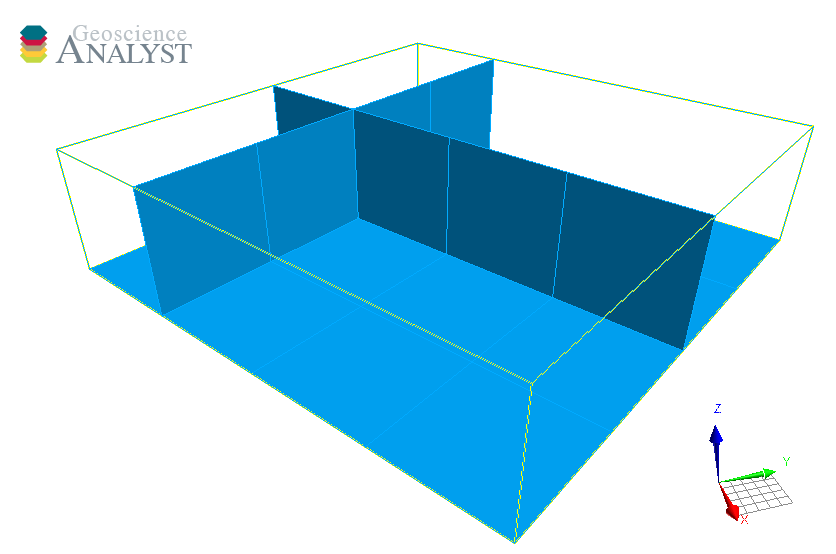
Octree

The Octree object is type of 3D grid that uses a tree structure to define cells. Each cell can be subdivided it into eight octants allowing for a more efficient local refinement of the mesh. The Octree object can also be oriented horizontally by controlling the rotation parameter.

from geoh5py.objects import Octree

octree = Octree.create(
        workspace,
        origin=[25, -100, 50],
        u_count=16,      # Number of cells in power 2
        v_count=32,
        w_count=16,
        u_cell_size=5.0, # Base cell size (highest octree level)
        v_cell_size=5.0,
        w_cell_size=2.5, # Offsets along z (down)
        rotation=30,
)

By default, the octree mesh will be refined at the lowest level possible along each axes.

workspace.close()