Data
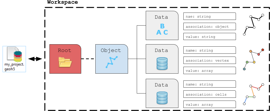
The geoh5 format allows storing data (values) on different parts of an Object. The data types currently supported by geoh5py are
Float
Integer
Text
Colormap
Well log
[1]:
from geoh5py.workspace import Workspace
import numpy as np

# Re-use the previous workspace
workspace = Workspace("my_project.geoh5")

# Get the curve from previous section
curve = workspace.get_entity("Curve")[0]
Float
Numerical float data can be attached to the various elements making up object. Data can be added to an Object entity using the add_data method.
[2]:
curve.add_data({
    "my_cell_values": {
        "association":"CELL",
        "values": np.random.randn(curve.n_cells)
    }
})
[2]:
<geoh5py.data.float_data.FloatData at 0x7f926c403d60>
The association can be one of:
OBJECT: Single element characterizing the parent object
VERTEX: Array of values associated with the parent object vertices
CELL: Array of values associated with the parent object cells
The length and order of the array of values must be consistent with the corresponding element of association. If the association argument is omited, geoh5py will attempt to assign the data to the correct part based on the shape of the data values, either object.n_values or object.n_cells
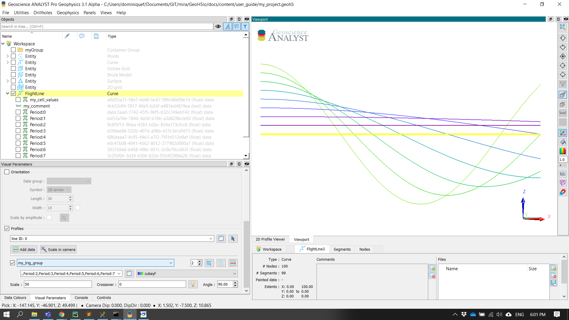
[3]:
# Add multiple data vectors on a single call
data = {}
for ii in range(8):
    data[f"Period:{ii}"] = {
        "association":"VERTEX",
        "values": (ii+1) * np.cos(ii*curve.vertices[:, 0]*np.pi/curve.vertices[:, 0].max()/4.)
    }

data_list = curve.add_data(data)
print([obj.name for obj in data_list])
['Period:0', 'Period:1', 'Period:2', 'Period:3', 'Period:4', 'Period:5', 'Period:6', 'Period:7']
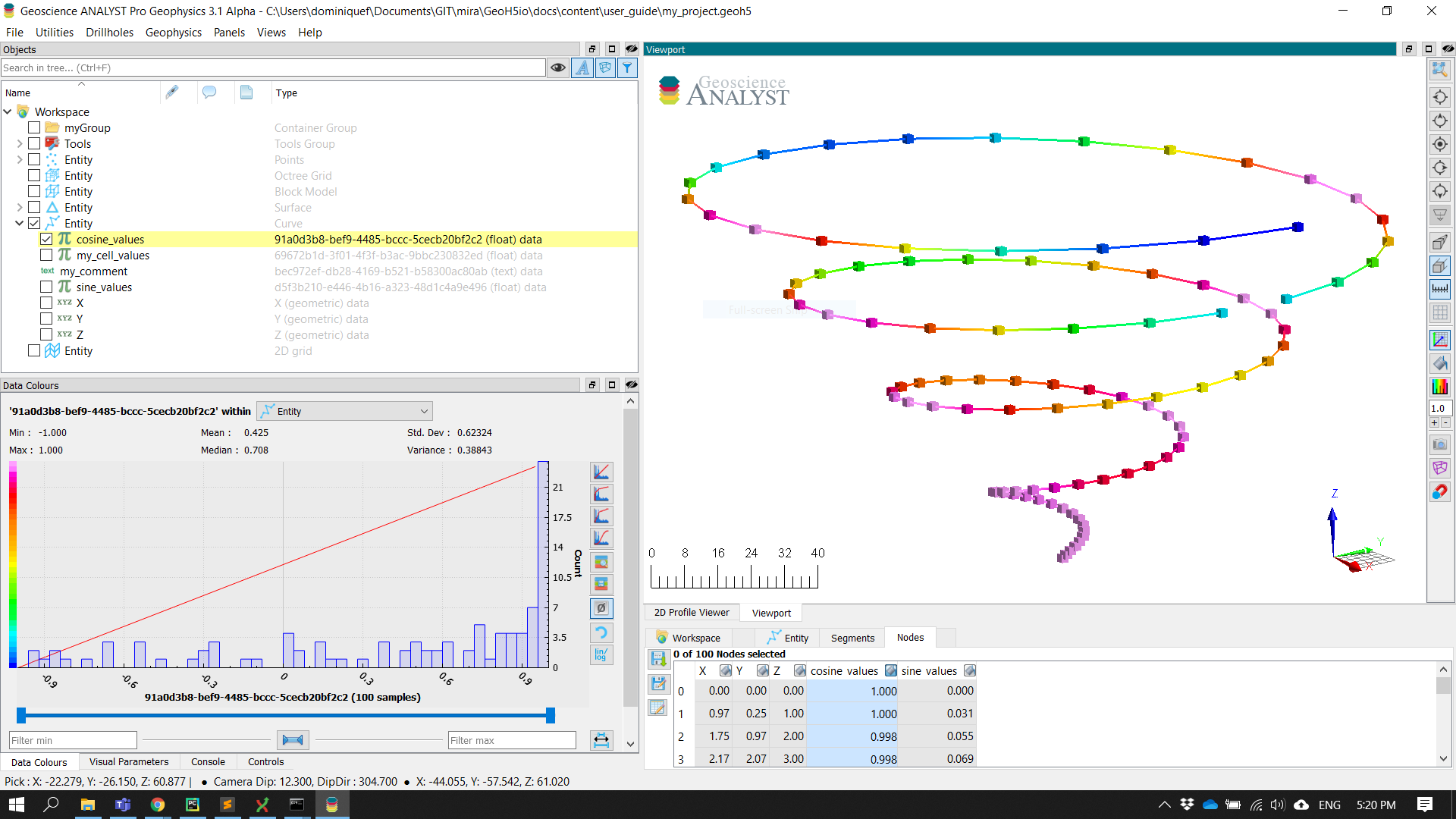
The newly created data is directly added to the project’s geoh5 file and available for visualization:
Integer
Same implementation as for Float data type but with values provided as integer (int32).
Text
Text (string) data can only be associated to the object itself.
[4]:
curve.add_data({
    "my_comment": {
        "association":"OBJECT",
        "values": "hello_world"
    }
})
[4]:
<geoh5py.data.text_data.TextData at 0x7f924153b9a0>
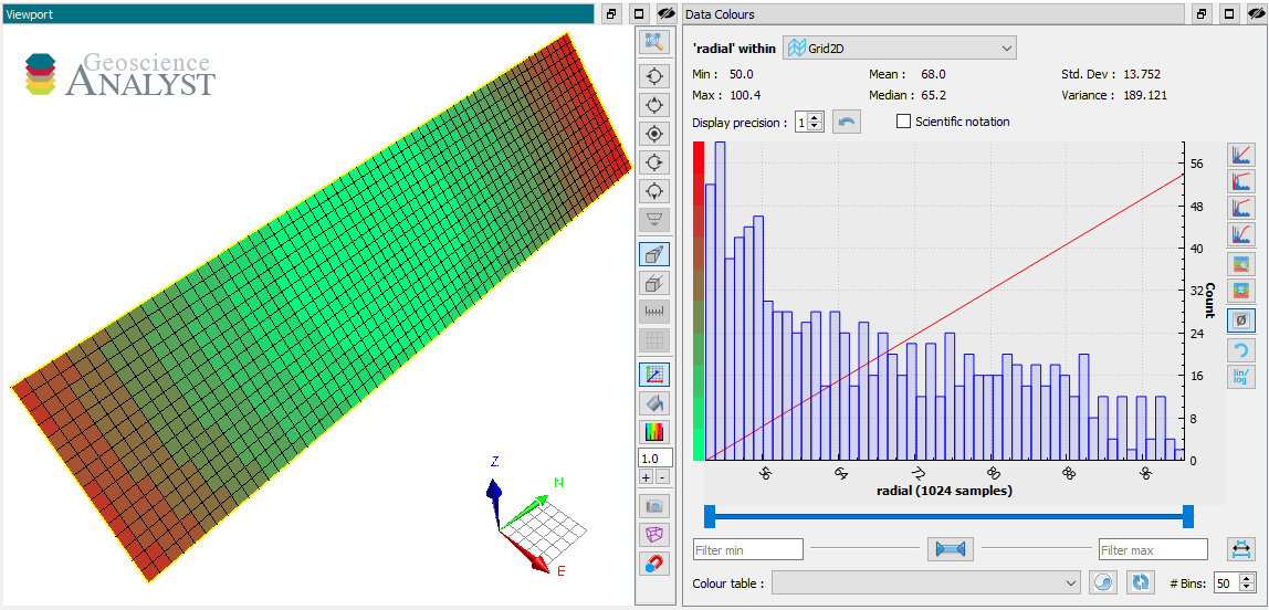
Colormap
The colormap data type can be used to store or customize the color palette used by Geoscience ANALYST.
[5]:
from geoh5py.data.color_map import ColorMap

# Create some data on a grid2D entity.
grid = workspace.get_entity("Grid2D")[0]

# Add data
radius = grid.add_data({
    "radial": {"values": np.linalg.norm(grid.centroids, axis=1)}
})
[6]:
# Create a simple colormap that spans the data range
nc = 10
rgba = np.vstack([
    np.linspace(radius.values.min(), radius.values.max(), nc), # Values
    np.linspace(0, 255, nc), # Red
    np.linspace(255, 0, nc), # Green
    np.linspace(125, 15, nc), # Blue,
    np.ones(nc) * 255, # Alpha,
]).T
We now have an array that contains a range of integer values for red, green, blue and alpha (RGBA) over the span of the data values. This array can be used to implicitly create a ColorMap from the EntityType.
[7]:
# Assign the colormap to the data type
radius.entity_type.color_map = rgba
The resulting ColorMap stores the values to geoh5 as a numpy.recarray with fields for Value, Red, Green, Blue and Alpha.
[8]:
radius.entity_type.color_map._values
[8]:
rec.array([( 56.32334484,   0, 255, 125, 255),
           ( 62.73899671,  28, 226, 112, 255),
           ( 69.15464858,  56, 198, 100, 255),
           ( 75.57030046,  85, 170,  88, 255),
           ( 81.98595233, 113, 141,  76, 255),
           ( 88.4016042 , 141, 113,  63, 255),
           ( 94.81725607, 170,  85,  51, 255),
           (101.23290795, 198,  56,  39, 255),
           (107.64855982, 226,  28,  27, 255),
           (114.06421169, 255,   0,  15, 255)],
          dtype=[('Value', '<f8'), ('Red', 'u1'), ('Green', 'u1'), ('Blue', 'u1'), ('Alpha', 'u1')])
Files
Raw files can be added to groups and objects and stored as blob (bytes) data in geoh5.
[9]:
file_data = grid.add_file("./c_data.ipynb")
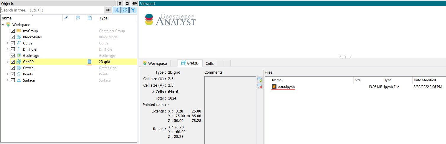
The information can easily be re-exported out to disk with the save method.
[10]:
file_data.save_file(path="./temp", name="new_name.ipynb")
Well Data
In the case of Drillhole objects, data are always stored as from-to interval values.
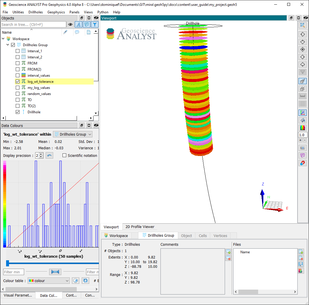
Depth Data
Depth data are used to represent measurements recorded at discrete depths along the well path. A depth attribute is required on creation. Depth markers are converted internally to from-to intervals by adding a small depth values defined by the collocation_distance. If the Drillhole object already holds depth data at the same location, geoh5py will group the datasets under the same PropertyGroup.
[12]:
well = workspace.get_entity("Drillhole")[0]
depths_A = np.arange(0, 50.) # First list of depth

# Second list slightly offsetted on the first few depths
depths_B = np.arange(0.01, 50.01)

# Add both set of log data with 0.5 m tolerance
well.add_data({
    "my_log_values": {
            "depth": depths_A,
            "values": np.random.randn(depths_A.shape[0]),
    },
    "log_wt_tolerance": {
            "depth": depths_B,
            "values": np.random.randn(depths_B.shape[0]),
    }
})
[12]:
[<abc.ConcatenatedFloatData at 0x7f926c4030d0>,
 <abc.ConcatenatedFloatData at 0x7f924153b8e0>]
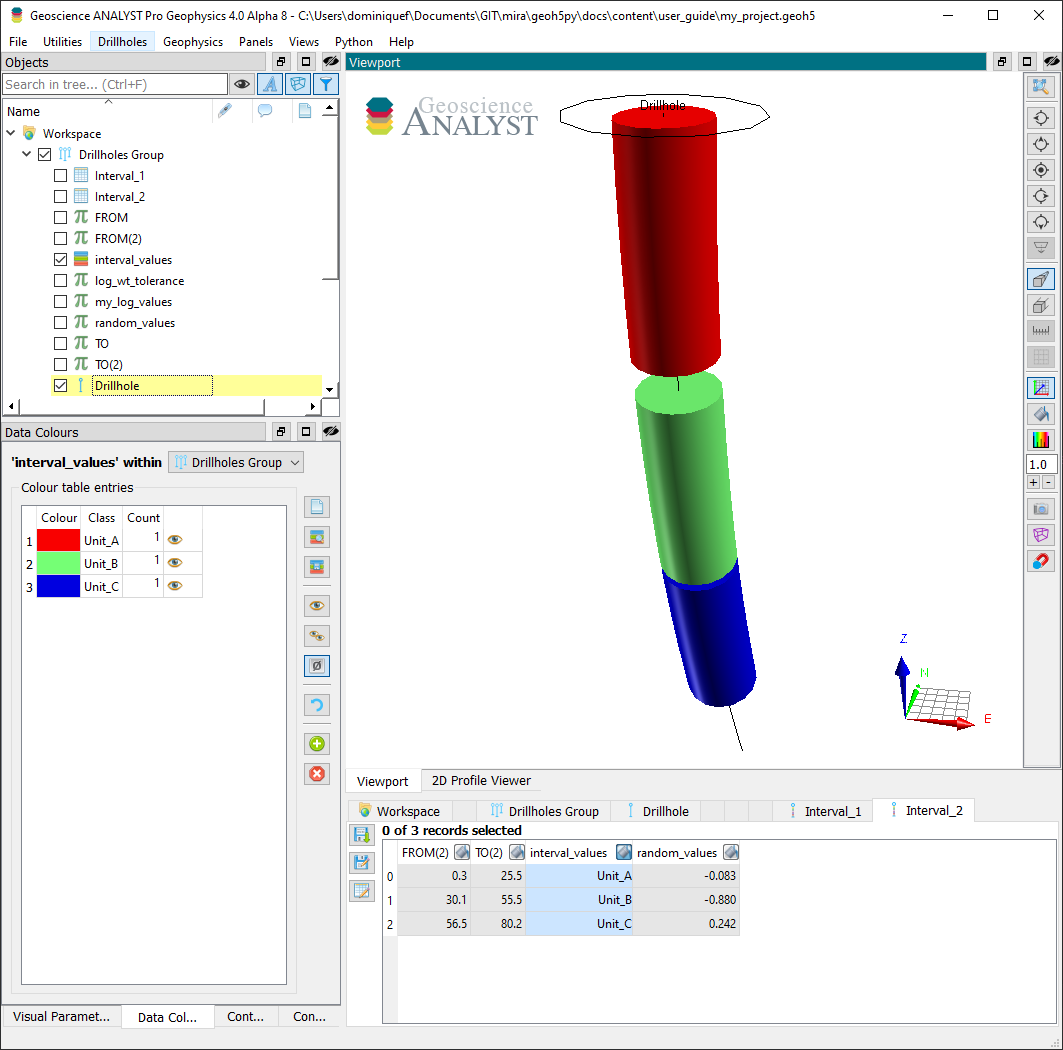
Interval (From-To) Data
Interval data are defined by constant values bounded by a start (FROM) and an end (TO) depth. A from-to attribute defined as a numpy.ndarray (nD, 2) is expected on creation. Subsequent data are appended to the same interval PropertyGroup if the from-to values match within the collocation distance parameter. Users can control the tolerance for matching intervals by supplying a collocation_distance argument in meters, or by setting the default on the drillhole entity
(default_collocation_distance = 1e-2 meters).
[13]:
# Define a from-to array
from_to = np.vstack([
    [0.25, 25.5],
    [30.1, 55.5],
    [56.5, 80.2]
])

# Add some reference data
well.add_data({
    "interval_values": {
        "values": np.asarray([1, 2, 3]),
        "from-to": from_to,
        "value_map": {
            1: "Unit_A",
            2: "Unit_B",
            3: "Unit_C"
        },
        "type": "referenced",
    }
})

# Add float data on the same intervals
well.add_data({
    "random_values": {
        "values": np.random.randn(from_to.shape[0]),
        "from-to": from_to,
    }
})
[13]:
<abc.ConcatenatedFloatData at 0x7f9241120bb0>
Get data
Just like any Entity, data can be retrieved from the Workspace using the get_entity method. For convenience, Objects also have a get_data_list and get_data method that focusses only on their respective children Data.
[14]:
my_list = curve.get_data_list()
print(my_list, curve.get_data(my_list[0]))
['Period:0', 'Period:1', 'Period:2', 'Period:3', 'Period:4', 'Period:5', 'Period:6', 'Period:7', 'my_cell_values', 'my_comment'] [<geoh5py.data.float_data.FloatData object at 0x7f926c403c10>]
Property Groups
Data entities sharing the same parent Object and association can be linked within a property_groups and made available through profiling. This can be used to group data that would normally be stored as 2D array.
[15]:
# Add another VERTEX data and create a group with previous
curve.add_data_to_group([obj.uid for obj in data_list], "my_trig_group")
[15]:
<geoh5py.groups.property_group.PropertyGroup at 0x7f924153a0b0>
[16]:
workspace.close()